Help
ChemSAR is a web-based platform for the rapid generation of quantitative
Structure‑Property and Structure‑Activity classification models
for small molecules. Starting from given structure of small molecules,
then, a step-by-step job submission process, ChemSAR will generate reliable and
robust predictive models.
In order to show the application of ChemSAR in generating models online, an example
is given in this page with detailed instructions and
screenshots. In this example, an dataset for building the toxic and non-toxic
chemicals classification model were taken from ( Cao D S, et al., 2015).
The data.csv contains the SMILES of each sample and the y.csv contains the SMILES
and the true label for each sample.
The following shows a detailed usage to establish a user customized model. All the
related files are listed in the
"Files and Download" section. All the related figures are listed at "Pictures"
section.
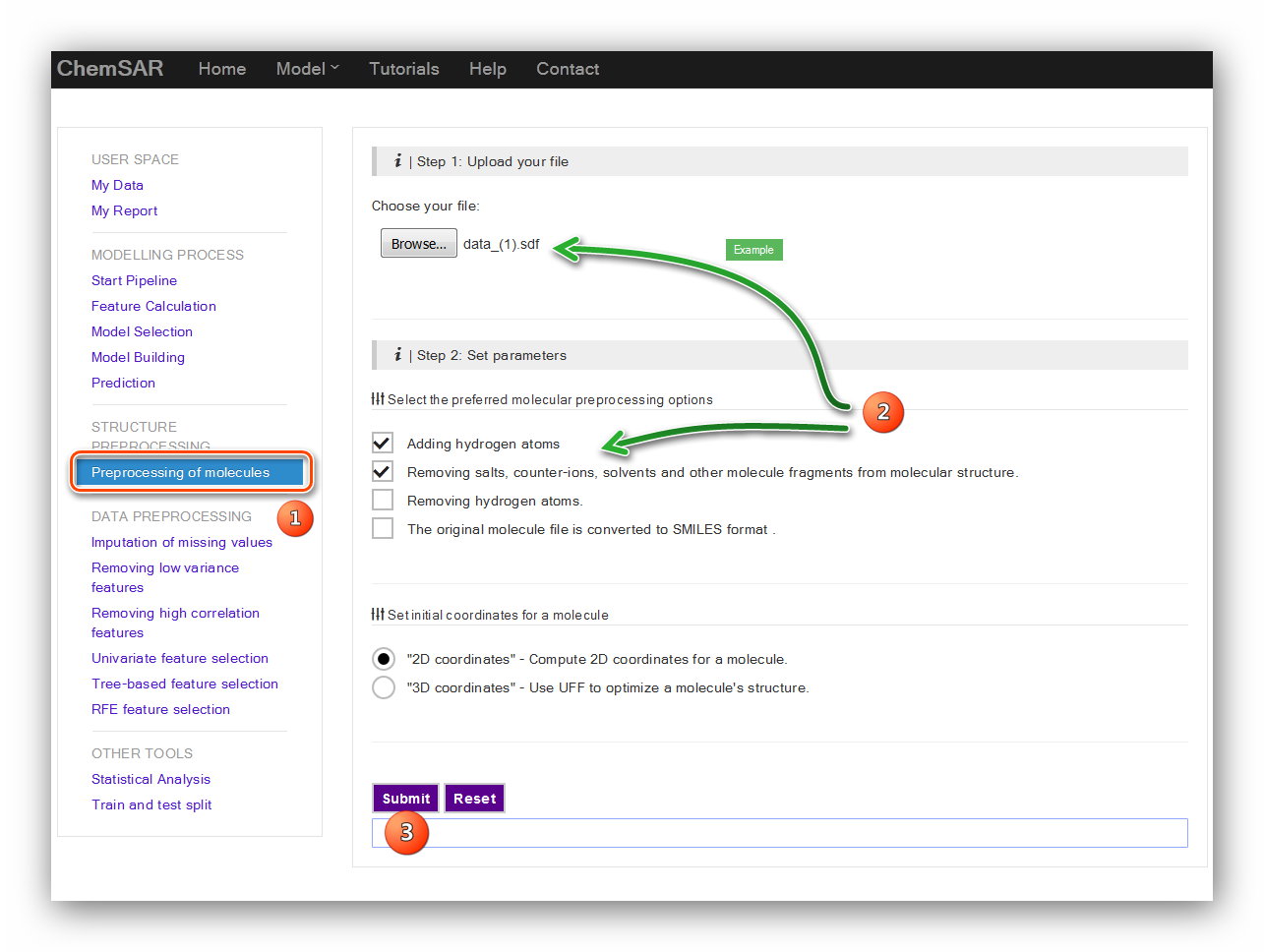
In this stage, a structure preprocessing will be applied to the molecules in File 1.
Six kinds of procedures can be selected by users
according to their initial molecular data including ‘Adding hydrogen atoms’,
‘Removing salts’, ‘Removing hydrogen atoms’, ‘converted to SMILES format’,
‘Compute 2D coordinates’ and ‘Compute 3D coordinates’. Here, we choose ‘Adding
hydrogen atoms’,
‘Removing salts’ and ‘Compute 2D coordinates’.(see Figure 1)
Input: File 1
Output: File 2
We need to start a job to use the whole modelling process. Click the “Start new job” button to get a unique job ID. (see Figure 2)
Here, ChemSAR enables users to compute 783 molecular descriptors and 10 kinds of
commonly used fingerprints. File 2, the output file of stage 1,
is uploaded and 194 features are calculated. These features include 30 constitution
descriptors, 35 topology descriptors,
7 kappa descriptors, 32 autocorrelation-broto descriptors, 5 molecular properties,
25 charge descriptors and 60 moe-type descriptors. (see Figure 3)
Input: File 2
Output: File 3
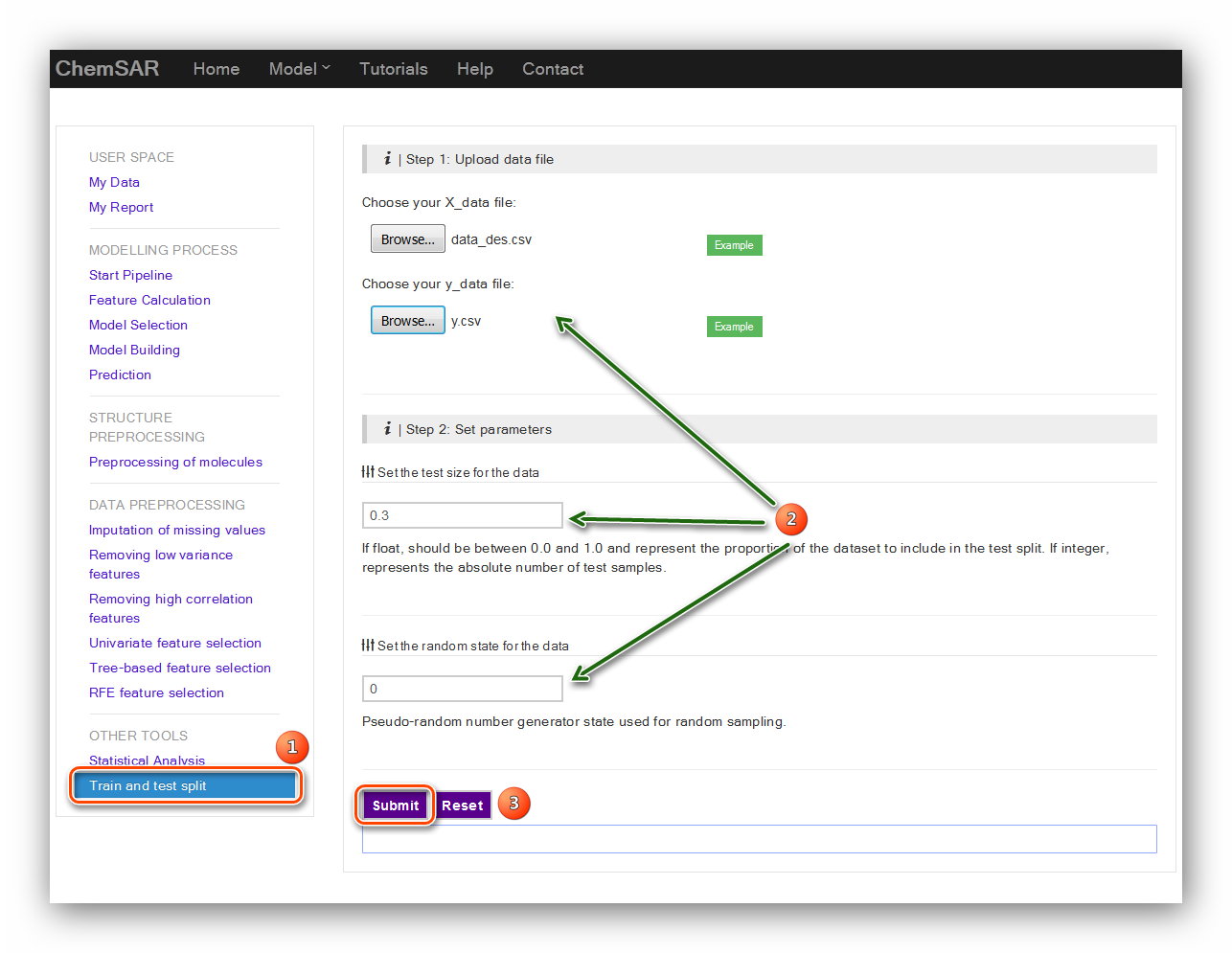
After the feature calculation stage, the data should be split into training set and
test set.
A random split into training and test sets can be quickly computed with the train
test split module.
There are two main parameters for this calculation: “test size for the data” and
“the random state”.
Their exact definitions are listed below the input form. Here,
we set 0.3 and 0 for the two parameters. (see Figure 4)
Input: File 4
Output: File 5, File 6, File 7, File 8
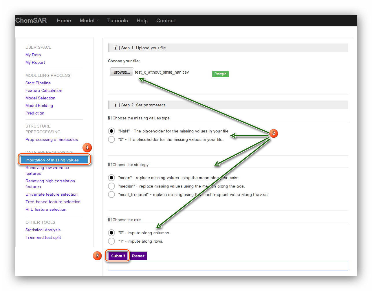
This module can be used to impute the missing values in you data. Check your File 5
and File 7. If some values are empty (nan) or gibberish, you can take this step and
impute the data. There are three parameters required: “the missing values type”,
“the strategy” and the axis. Also, the exact definitions about these parameters are
listed below the input form. Here, we find the value in column 39, index 35 is
“-inf”. This value is not correct or cannot be recognized by built-in functions. In
order to give a clearer picture of how to impute the data, we have manually removed
several values randomly include the values mentioned above. (File 7 to File 9).
Then, we use the default values for the parameters.
(see Figure 5) Likewise, if other related data exists missing values you
should also take this step to ensure an up-to-standard data.
Input: File 9
Output: File 10
This is a simple baseline approach to feature selection. It removes all features
whose variance doesn’t meet some threshold. By default,
it removes all zero-variance features.
Features with a variance lower than a threshold will be removed.
Here, we set the threshold as 0.05. (see Figure 6)
Input: File 11 (delete the column: SMILES of File
5)
Output: File 12
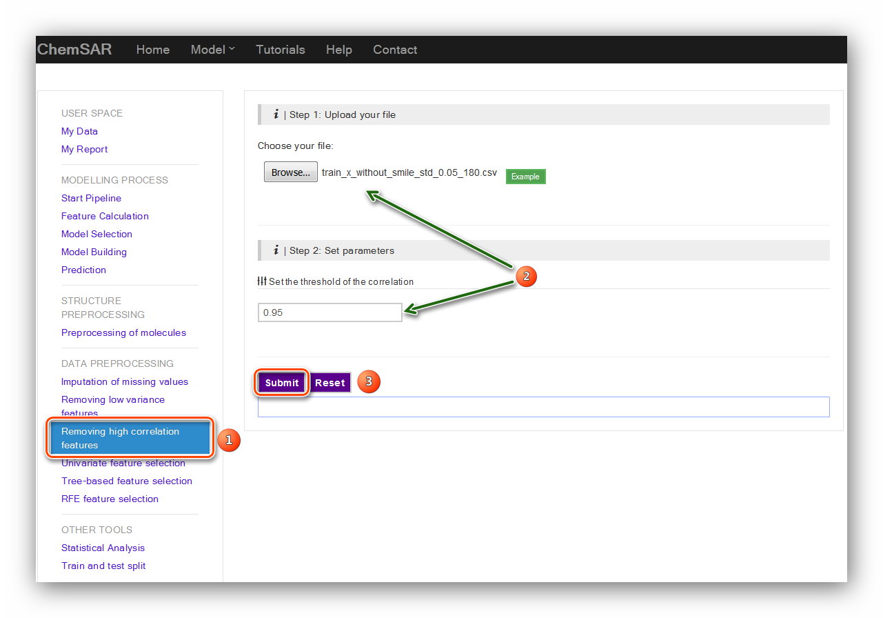
Removing high correlation features is another useful baseline approach to feature
selection.
It removes all features whose correlation doesn’t meet some threshold. Here, we set
the threshold as 0.95. (see Figure 7)
Input: File 12
Output: File 13
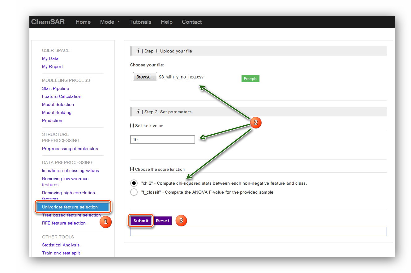
Univariate feature selection works by selecting the best features based on
univariate statistical tests.
It can be seen as a preprocessing step to an estimator. It removes all but the k
highest scoring features.
Here, we set the k value as “10” and the score function as “chi2”. In order to use
“chi2” function we have
manually removed the features contain negative values (This is just for an example).
At the same time we added the y_true column (From File 6) to the end of the file.
These two steps turn File 13 into File 14.
(See Figure 8)
Feature importances can be computed by tree-based estimators. which in turn can be
used to discard irrelevant features. This module employs a meta estimator that fits
a number of randomized decision trees on various sub-samples of the dataset and use
averaging to improve the predictive accuracy and control over-fitting. There are
three parameters required for the calculation.
Their exact definitions are listed below the input form. Here, we use the default
parameters to process. (See Figure 9 and Figure 10)
Input: File 15(add y_true column to File 14 and get
File 15)
Output: File 16
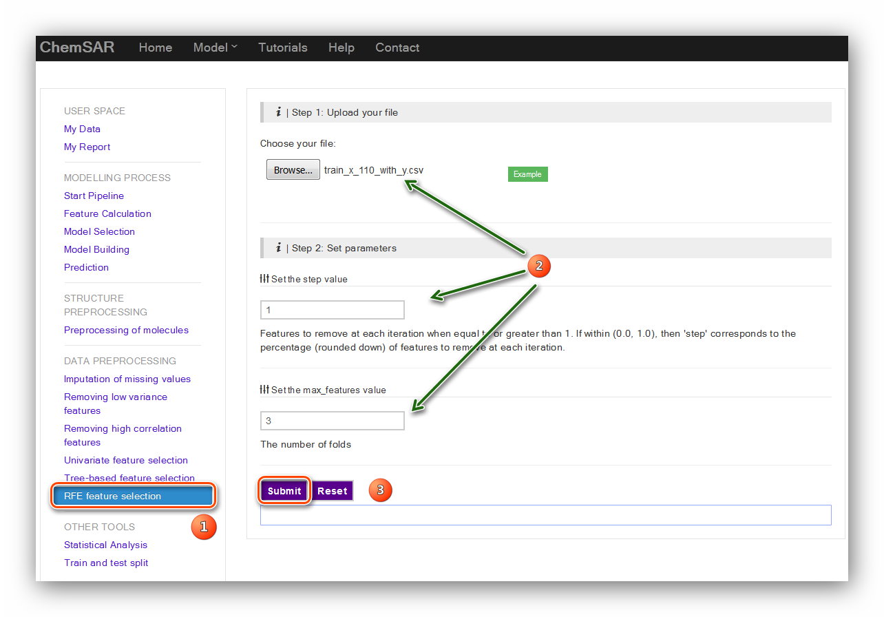
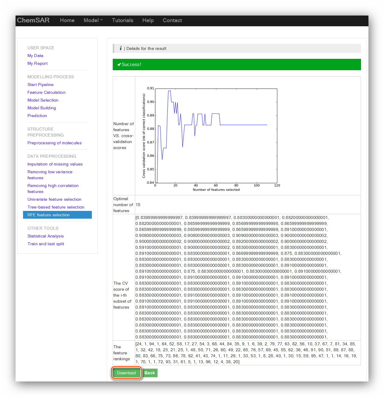
Recursive feature elimination (RFE) is to select features by recursively considering
smaller and smaller sets of features. First, the estimator is trained on the initial
set of features and weights are assigned to each one of them. Then, features whose
absolute weights are the smallest are pruned from the current set features. That
procedure is recursively repeated on the pruned set until the desired number of
features to select is eventually reached. In this module, RFE is performed in a
cross-validation loop to find the optimal number of features and the support vector
classification estimator with a linear kernel is utilized to process. There are two
parameters required:
step value and the fold value. Their definitions are listed below the input forms.
Here,
we use the default parameters. (See Figure 11 and Figure 12)
Input: File 15
Output: File 17
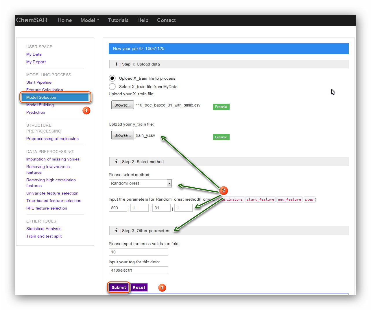
In order to give an overall report for the whole modelling pipeline, a unique job ID
is needed and should be created in stage 2.
All the results from each step of modelling will be attached to this job ID. In this
module, there are 5 kinds of commonly used machine learning methods available.
They are “Random Forest”, “Support Vector Machine”, “Naïve Bayes”, “K Neighbors” and
“Decision Tree”. Each method requires several parameters for the calculation.
For some ones that need a parameter optimization, a general grid search method is
utilized to perform. Here, take the “Random Forest” method for an example.
We set the parameters as follows: ‘n_estimators’: 800, ‘step’: 1, ‘end_feature’: 31,
‘start_feature’: 1, ‘cv’: 10. The data tag for the data
is just a mark for
the file you uploaded and it is helpful when you check your data in the “My Data”
module. The model tag for the model
is a mark for
the model you established currently and it is helpful when you check your models in the “My Model”
module. Here, we type in “418selectrf” (See Figure 13).
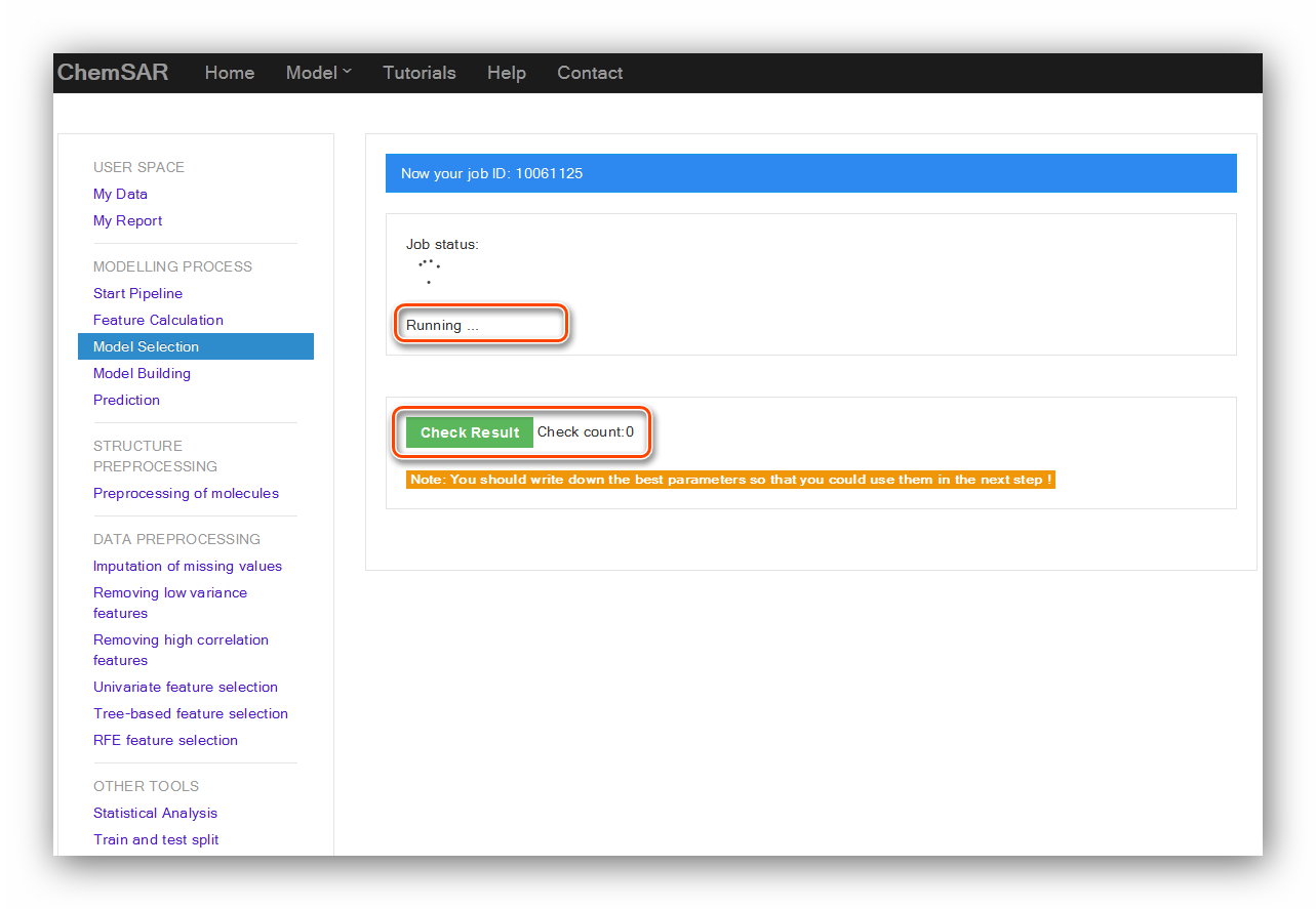
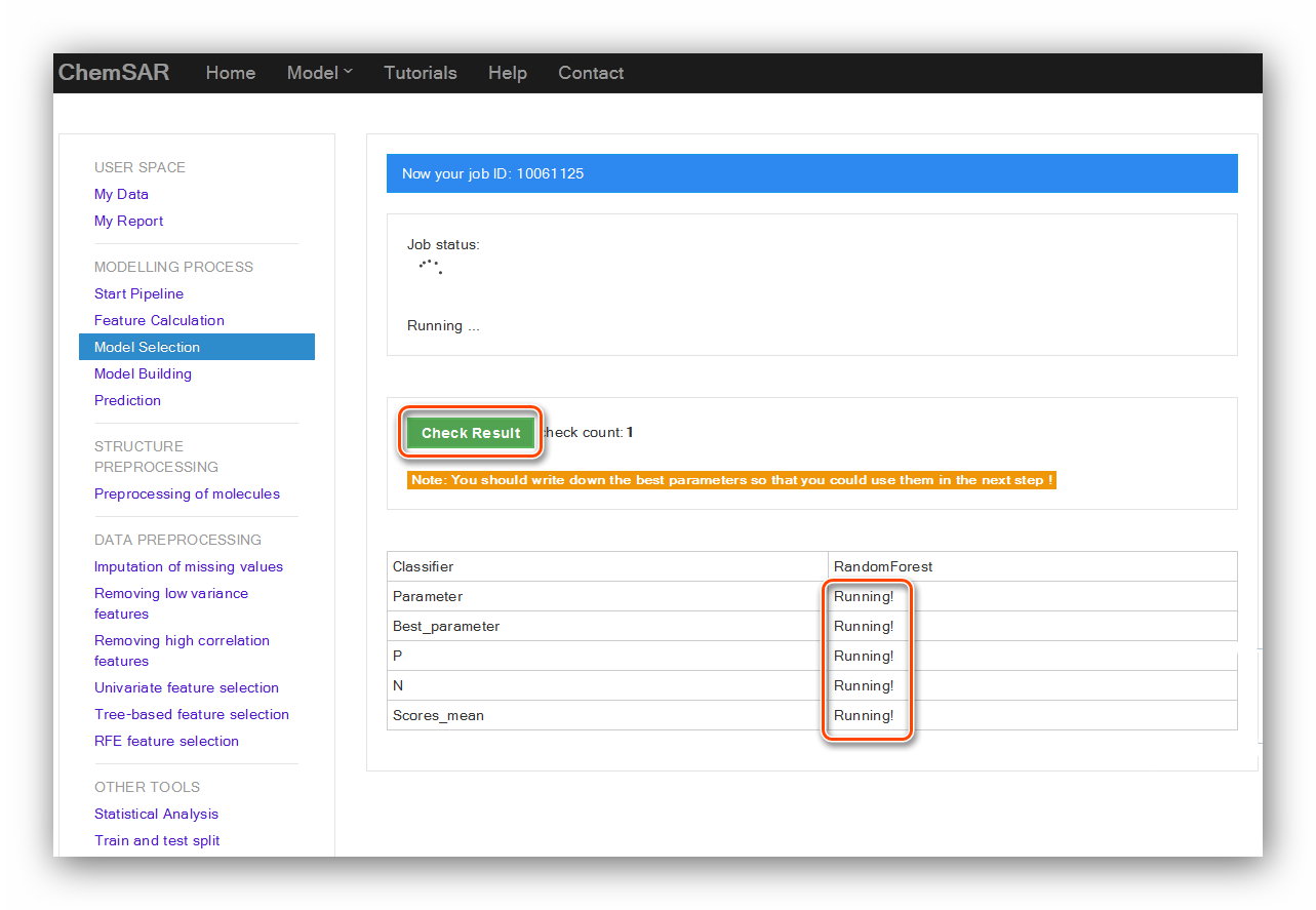
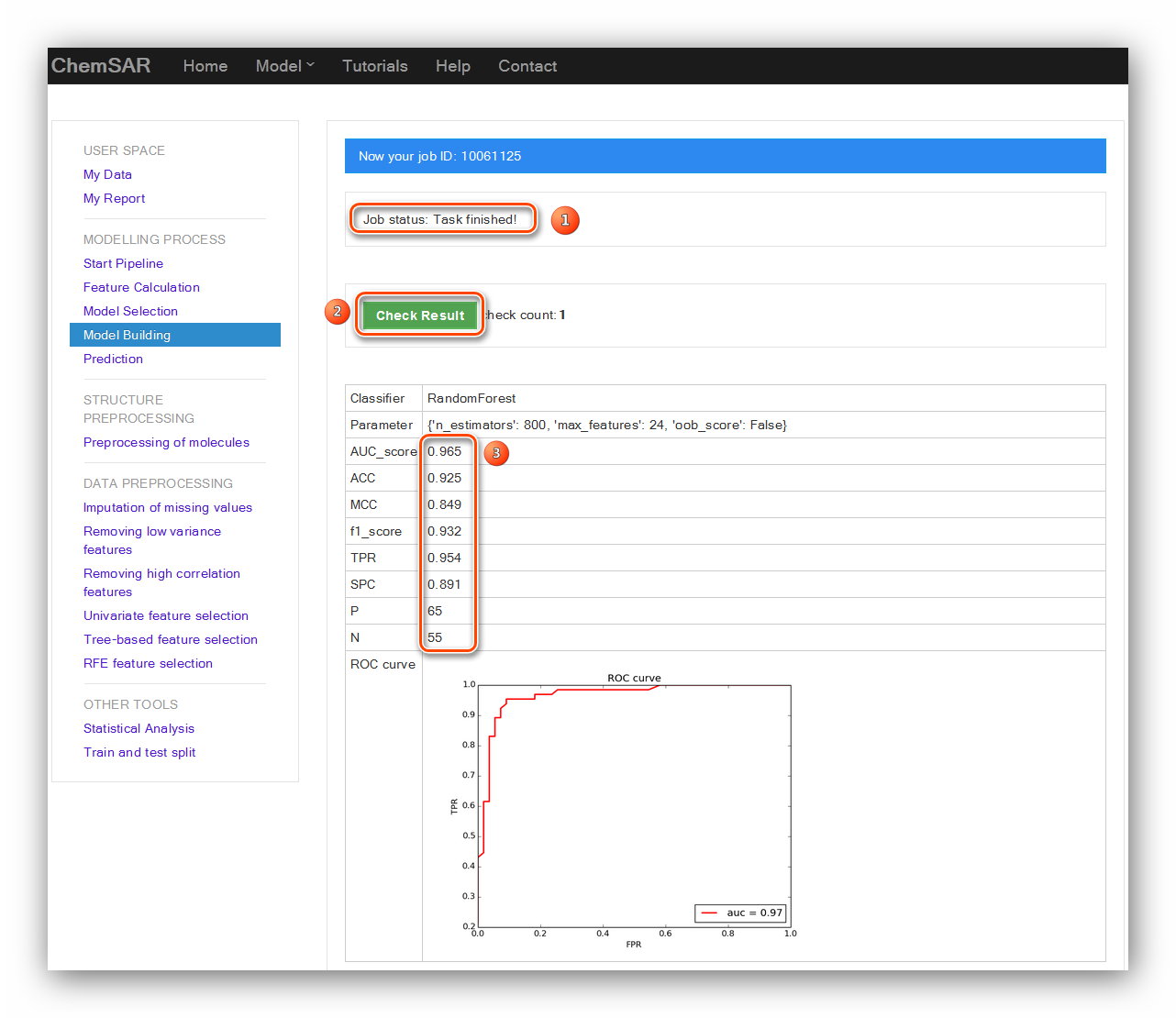
The calculation process will last for a while according to the data and method users
selected. After clicking the “Submit” button,
you will be redirected to the result page (See Figure 14). There, you can
check your job status. After the completion of the calculation,
click “Check Result” button again, the result
contents will be displayed in the page (See Figure 15 and Figure 16).
Since we use “session” and “AJAX” technique,
there will be no “Time out (504 error)” any more. You can check your job status at
any time at this page. Even, you can close your browser or shut down your
computer and check the results according to the job ID at the “My Report” module.
This is very convenient for users to accomplish a multi-step and time-consuming
task.
Input: File 18(Add the smile column to File 16 and
get File 18) and File 6
Output: Results in the page.
In the “Model Selection” stage, you have tried a series of methods and their
parameters. Finally, you get a set of best parameters for your data.
In this stage, you should input the method and the best parameters. Then, a reliable
and desired model will be established.
The results will be displayed in the result page and the model itself will be dumped
into files for the use of “Prediction” module (See Figure 17 and Figure
18).
Input: File 18 and File 6
Output: Results in the page.
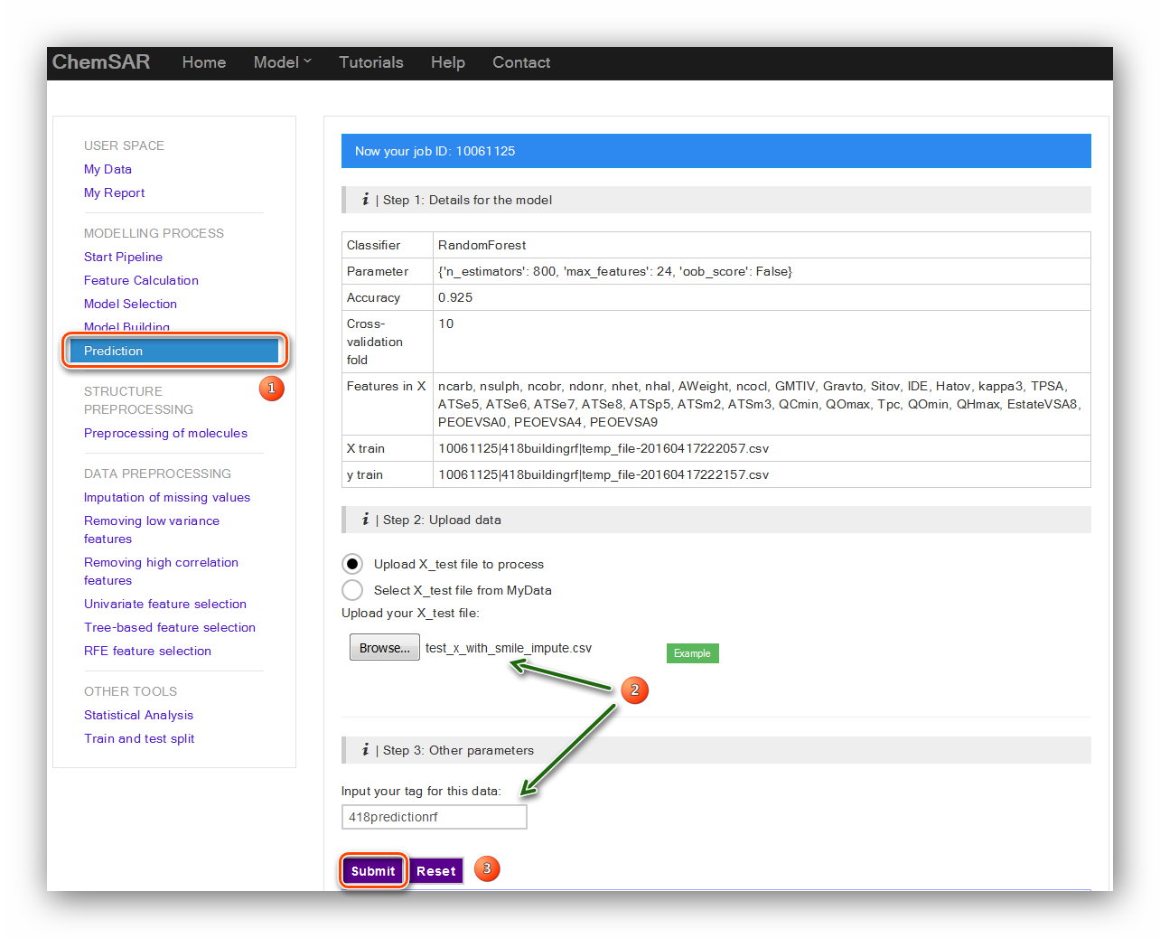
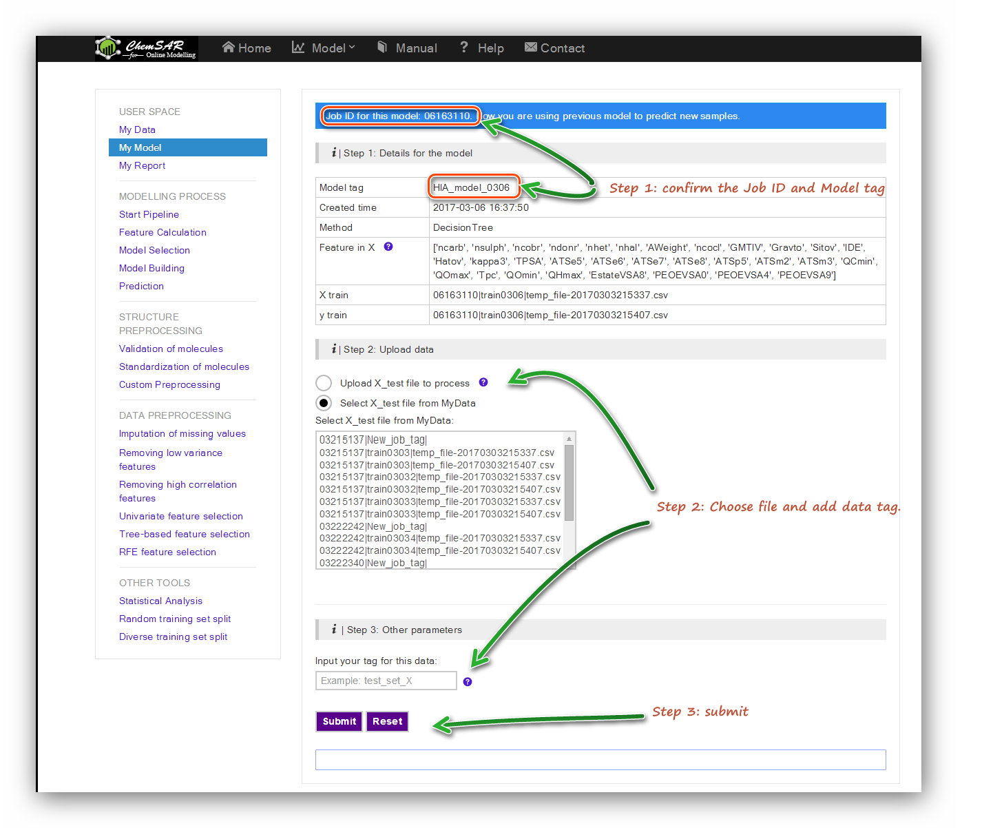
In the “Model Building” stage, a reliable model has been established according to
your requirements and has been saved temporarily.
In the index page of this module, you will see a table contains the related
information from the “Model Building” stage.
Check the information and upload test set file to process if the information is
correct. Here, we add the smile column to the start of File 10,
and then we get File 19. Note that an automatic indexer will be employed to pick up
the right feature columns (Features in X) of the uploaded file.
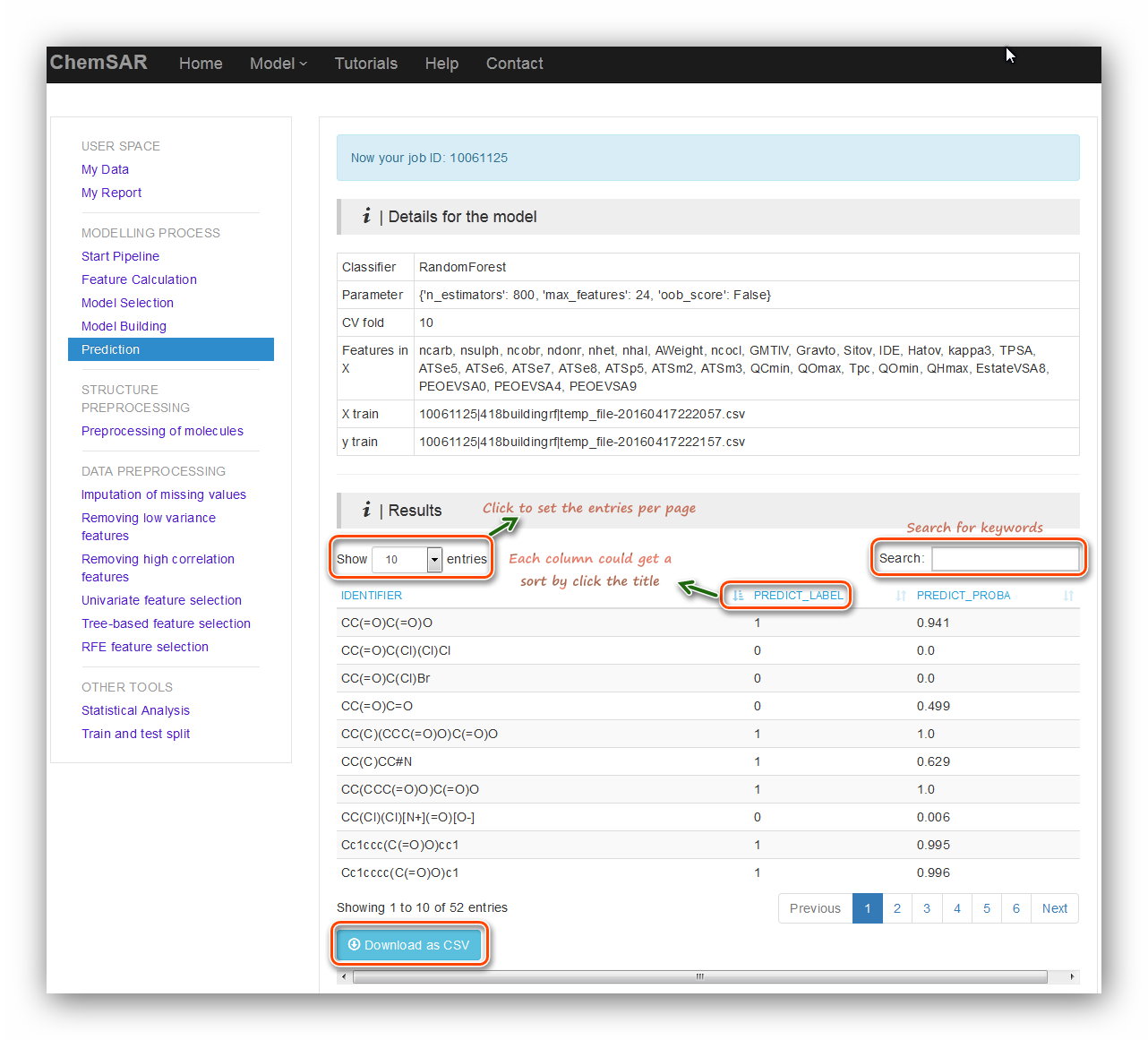
Click the “Submit” button to start the prediction (See Figure 19). In the
result page, an interactive table contains prediction results will be displayed.
Several table tools are available for you to get what you want.
At the bottom, a “Download as csv” button is for you to download the results (See
Figure 20).
Input: File 19
Output: File 20
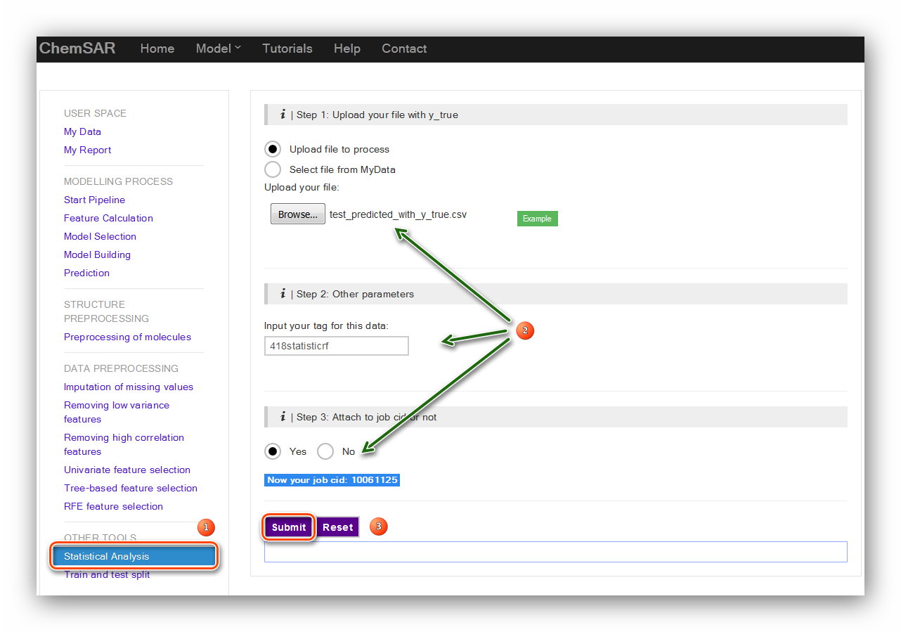
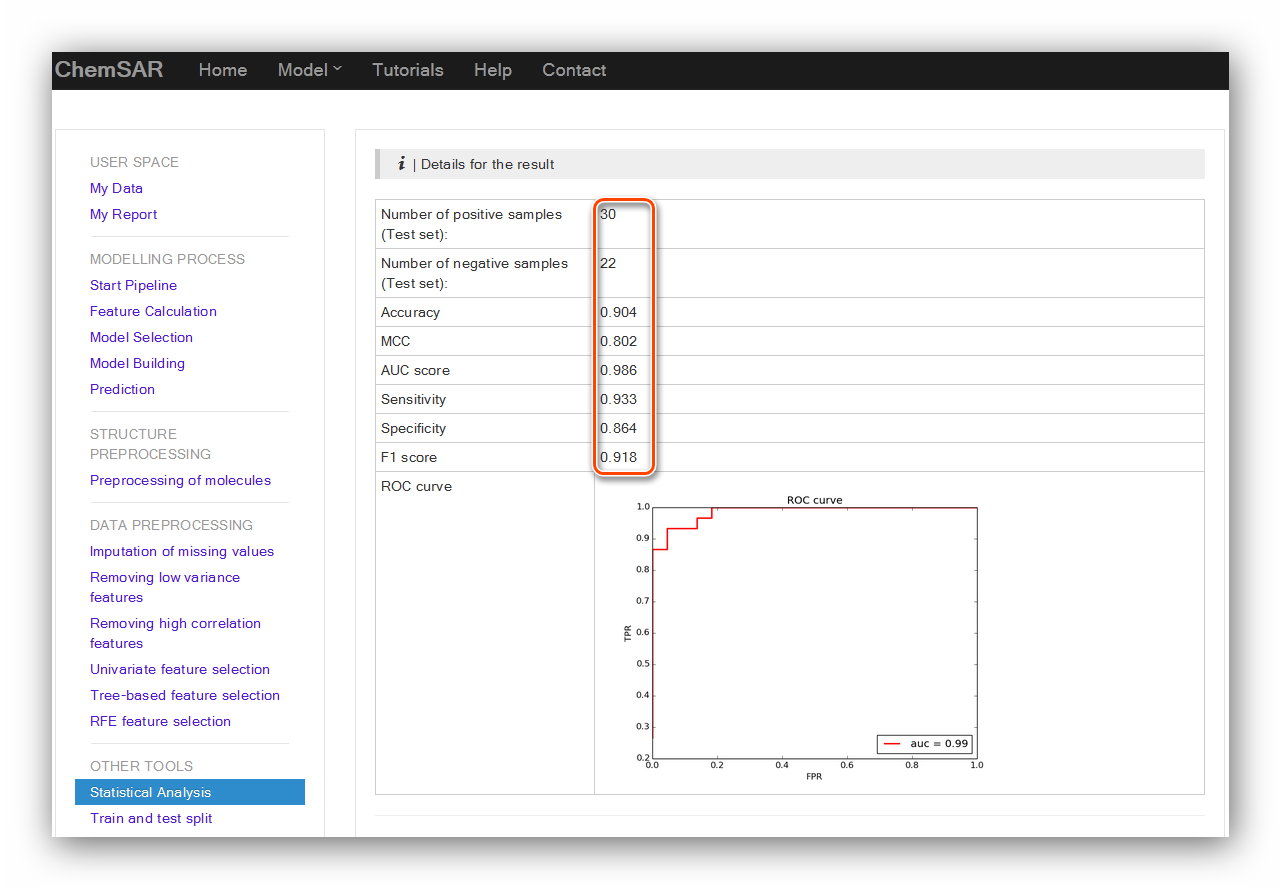
If you have a test set for the model like in this example. Another selectable tool:
“Statistical Analysis” is there for you to assess the performance of
the model using the external test set. After the prediction, add the “y_true” column
from File 8 to the end of File 20, and then we get File 21.
Upload the File 21 and click the “Submit” button and we will be redirected to the
result page (See Figure 21 and Figure 22).
Input: File 21
Output: Results in the page.
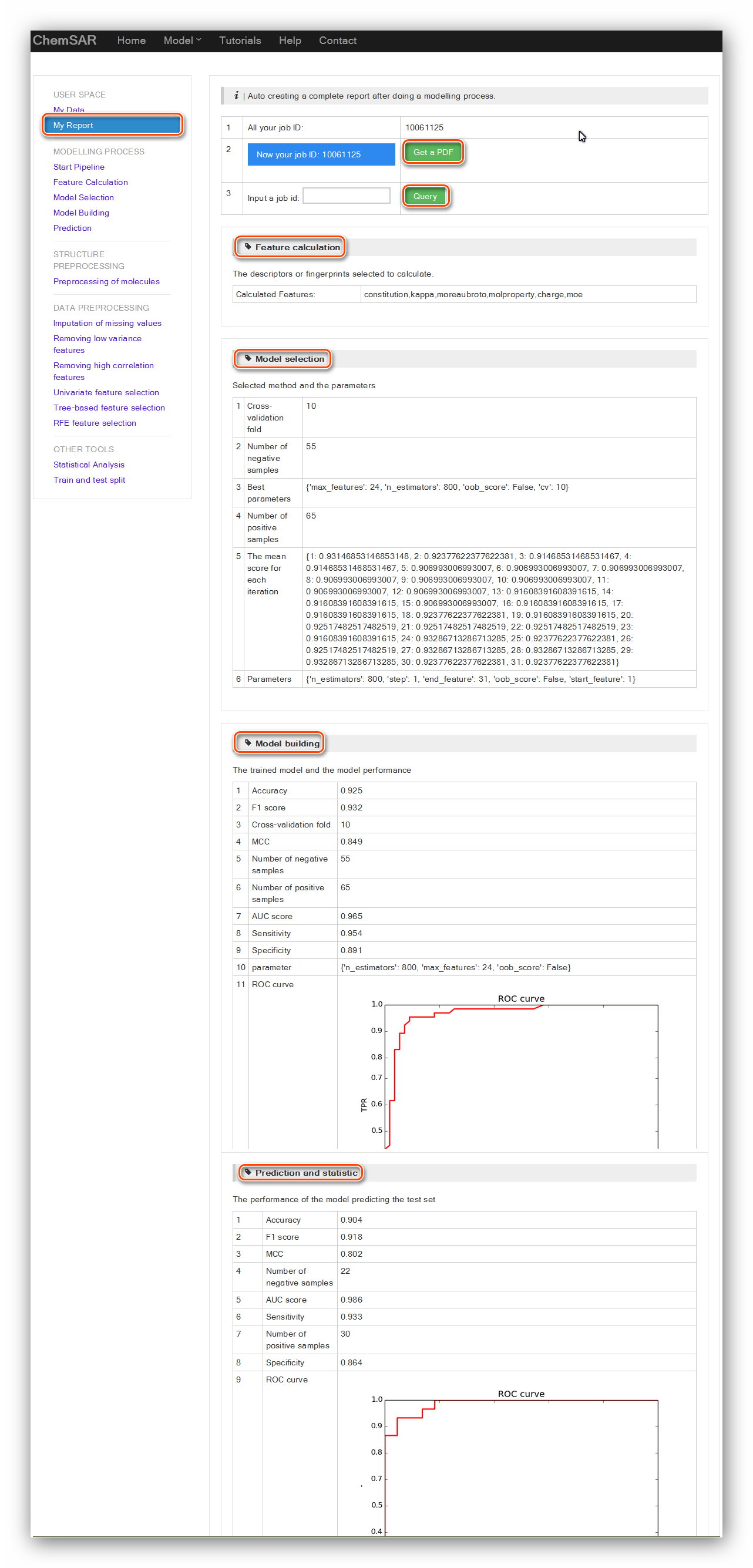
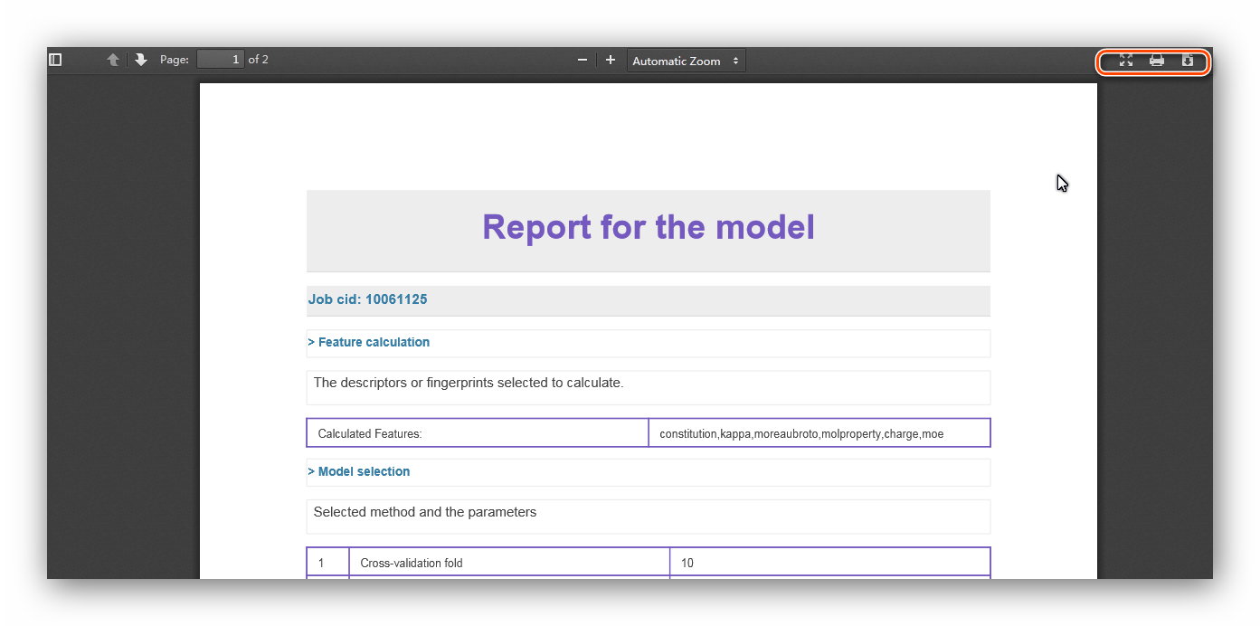
A specific feature of ChemSAR is that it provides a complete report generation
system.
It retrieves result data of each calculation and transforms them into a HTML page
and a PDF file for users.
After finishing going through the whole modelling pipeline, you can go to “My
Report” module to obtain a well-organized
report including information from “Feature Calculation” to “Prediction and
statistic” (See Figure 23). At the index page of this module,
all the job IDs that you have started will be listed there. A “Get a PDF” button
allows you to generate a PDF for an off-line usage.
A “Query” button is available for you to query the
information about models created in other jobs.
This is also very helpful when you attempt to building models using different
methods and parameters or
when you want to build more than one model at the same client at the same time (See
Figure 24).
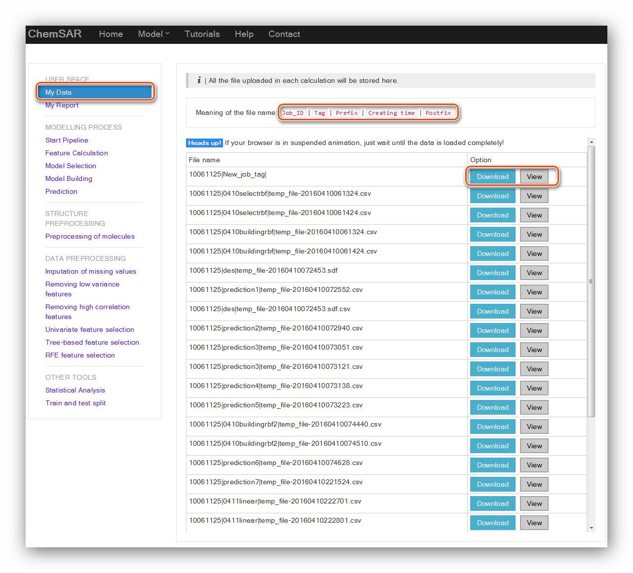
A file system that allows users to view files they uploaded in each step according
to the tags users could reuse these files conveniently.
In the index page, a file name meaning is explained. Once users upload a file, it
will be stored in the user space and the file name will be listed in the table.
The “Download” and “View” buttons allow users to download the file for reuse and
view the file content. (See Figure 25)
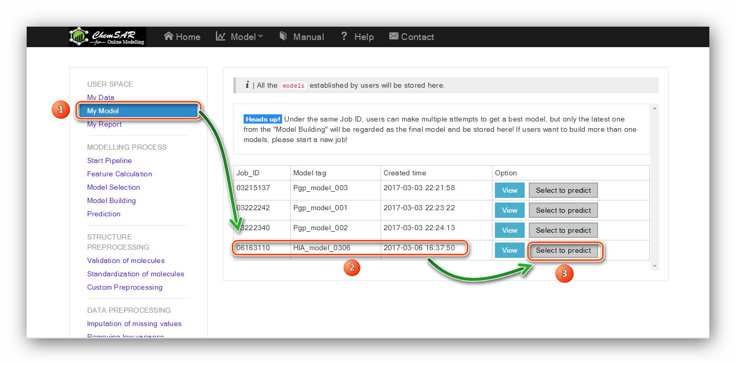
A file system that used to store all the models built in the "Model building" stage.
Under the same job ID, users can make multiple attempts to get a best model,
but only the latest one from the "Model Building" will be regarded as the final model and be stored here!
If users want to build more than one model, please start a new job!
Users can start several jobs(Max: 10) to build different models. If all the 10 job IDs run out, users should
delete the browser cookies (sessionid from http://chemsar.scbdd.com), and come back as a new guest user, or
change for a new client.
(See Figure 26, 27)
Click the picture to see big one, and click again to go back.


The recommended browsers: Safari, Firefox, Chrome, IE(Ver. >8).
 E-mail: jiedong@csu.edu.cn
 |
 |
 |
 |
|
 |