Manual
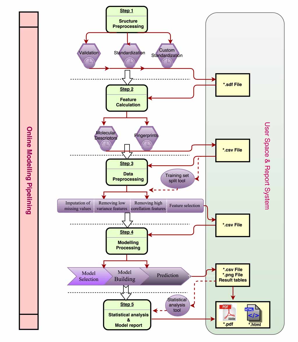
| Overview and a suggested pipelining
| Input & output formats
The table below listed requirements of formats for each module, and users should prepared data files as following before calculation.
| Module name | Input | Output | Description | Sketch |
|---|---|---|---|---|
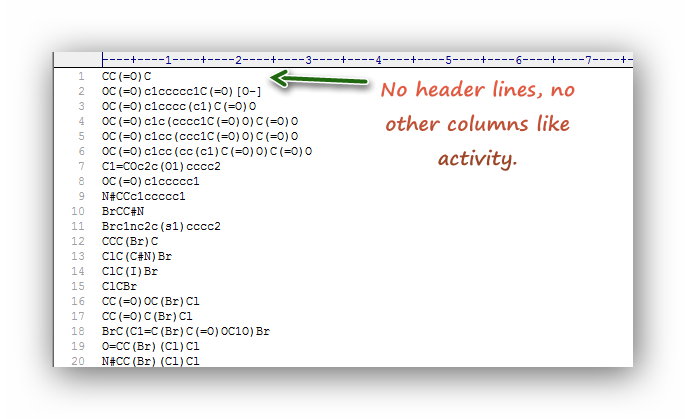
| Feature calculation | *.smi; *.sdf | *.csv | The de facto standard version of molfile in SDF must be V2000; 2D or 3D information are both valid; The first row of *.csv file is the descriptor names; the first column is the SMILES of molecules. | *.smi file *.sdf file |
| Model selection | *.csv | data table in the page | The first column of X_train file can be molecular symbol like molecular names or IDs; the first row of X_train file must be descriptor names; the first column of y_train file must be the same with X_train file; the second column must be experimental value of the sample(different presentation styles of classes must be convert into 0 or 1 ). | X train file y train file |
| Model building | *.csv | data table in the page; *.png | The same with "Model selection". | X train file y train file |
| Prediction | *.csv | data table in the page; *.csv | The requirements of X_test file is the same with X_train file. | X test file |
| Validation of molecules | *.sdf | *.csv | The de facto standard version of molfile in SDF must be V2000. | *.sdf file |
| Standardization of molecules | *.sdf | *.sdf | The same with "Validation of molecules". | *.sdf file |
| Custom preprocessing | *.sdf | *.sdf | The same with "Validation of molecules". | *.sdf file |
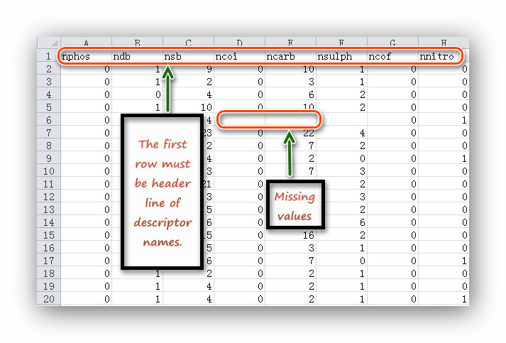
| Imputation of missing values | *.csv | *.csv | The first row of input file must be header like descriptor names; each column including the first one must be feature values like descriptor values. | *.csv file |
| Removing low variance features | *.csv | *.csv | The same with "Imputation of missing values". | *.csv file |
| Removing high correlation features | *.csv | *.csv | The same with "Imputation of missing values". | *.csv file |
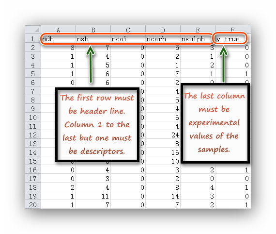
| Univariate feature selection | *.csv | *.csv | The first row of input file must be header like descriptor names; each column from the first one to the penultimate one must be feature values like descriptor values; The last column must be experimental value of the sample(different presentation styles of classes must be convert into 0 or 1 ). | *.csv file |
| Tree-based feature selection | *.csv | data table in the page; *.csv | The same with "Univariate feature selection". | *.csv file |
| RFE feature selection | *.csv | data table in the page; *.csv; *.png | The same with "Univariate feature selection". | *.csv file |
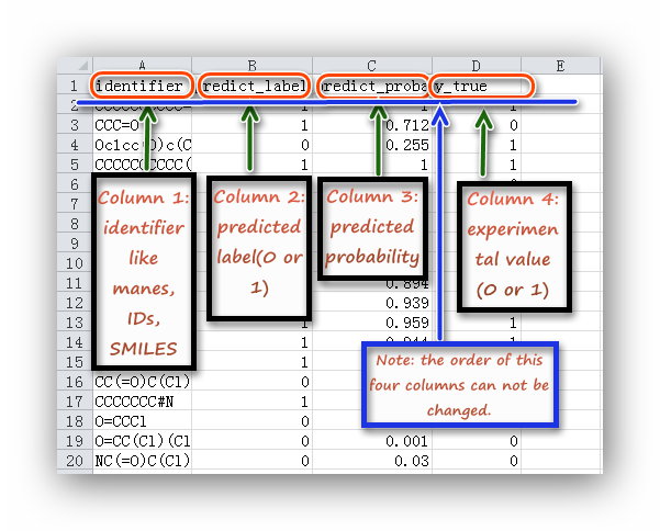
| Statistical analysis | *.csv | data table in the page; *.png | The four columns of input file must be in order: molecular identifier,predict label,predict probability,experimental value; the label name can be defined by users. | *.csv file |
| Random training set split | *.csv | *.csv | The same with "Model selection". | X data file y data file |
| Diverse training set split | *.sdf | *.sdf | The de facto standard version of molfile in SDF must be V2000; 2D or 3D information are both valid. | *.sdf file |
| Feature importance | *.csv | *.csv | The same with "Univariate feature selection". | *.csv file |
| Algorithms and parameters
ChemSAR now provides five main algorithms for building classification models. The algorithms along with their main parameters that need to be optimized are listed in the table below.
| Algorithms | Parameters | Recommended parameters |
|---|---|---|
| RandomForest | n_estimators: The number of trees in the forest; | n_estimators:500; |
| max_features: The number of features to consider when looking for the best split; (start_feature, end_feature and step make up the attempts of max_features) | max_features: sqrt(N); N stands for number of features; | |
| cv: cross validation fold | cv: 5 | |
| SVM | kernel type: rbf, sigmoid, poly, linear; | |
| C: penalty parameter C of the error term.; | C: 2^-5, 2^15, 2^2; (format: start, end, step) | |
| gamma: kernel coefficient for 'rbf', 'poly' and 'sigmoid'; | gamma: 2^(-15), 1, 2^2; | |
| degree: degree of the polynomial kernel function; | degree: 1, 7, 2 | |
| cv: cross validation fold | cv: 5 | |
| Naïve Bayes | Bayes classifier type; | BernoulliNB for binary-valued variable; GaussianNB for continuous variable |
| cv: cross validation fold | cv: 5 | |
| K Neighbors | n_neighbors: number of neighbors to use; | n_neighbors: 1-10; |
| cv: cross validation fold | cv: 5 | |
| DecisionTree | Algorithm: algorithm used to compute the nearest neighbors ('ball_tree', 'kd_tree', 'brute'); | automatic decision; |
| cv: cross validation fold | cv: 5 |
| Theory and how to choose a proper algorithm
In ChemSAR, we implemented five learning algorithms by now. The following is a brief description of each algorithm. Users can decide which one to choose according their purposes and datasets.
Random forest (RF) is proposed by Breiman at 2001, which uses an ensemble of classification trees. Each tree in the ensemble is constructed using a different bootstrap sample of the data. In addition, when constructing trees, each node is split using the best feature among a subset of predictors randomly chosen at that node instead of using the best split among all variables. Due to this randomness, the bias of the forest usually slightly increases, while the variance also decreases for the averaging strategy. These strategies make RF algorithm have excellent performance in classification tasks. In building SAR classification models, it is suitable for dataset with many more features than observations and dataset with some noisy features. During the RF model selection, two main parameters (mtry and ntree) need to be optimized to achieve excellent performance. The mtry is the number of input variables tried at each split which is very important. The ntree means that how many trees to grow for each forest. To get a set of good parameters, a grid search strategy is used by inputting n_estimators, start_feature, end_feature and step in the corresponding submitting page. The n_estimators represent ntree, and the start_feature, end_feature and step make up the attempts of mtry. In addition, a k-fold cross validation process was implemented to assess the model performance, so a parameter cv (cross validation fold) is required for this calculation.
Support Vector Machine (SVM) was proposed by Vapnik and his coworkers. The optimal separating hyperplane strategy makes SVM have many nice statistical properties, which greatly accelerate the expansion of the SVM and the applications in a variety of fields. To obtain a good SVM model for classification, a set of parameters should be selected depending on the selection of kernel. Among these parameters, kernel type is the kernel type to be used in the SVM algorithm. It must be one of linear, poly, rbf and sigmoid. If rbf type is chosen, the ranges of C (the penalty parameter of the error term) and gamma (the kernel coefficient) are required to be set; if linear type is chosen, the range of C is required; if poly type is chosen, the ranges of C, gamma and degree (the degree of the polynomial kernel function) are required; if sigmoid is chosen, the ranges of C and gamma are required to be set. Then a grid search strategy will be employed to identify the optimal combination of their corresponding parameters. Besides, the parameter cv (cross validation fold) is also required for this calculation.
Naive Bayes (NB) has been studied extensively since the 1950s, which are a set of supervised learning algorithms based on applying Bayes’ theorem with the “naive” assumption of independence between every pair of features. NB works quite well in many real-world situations and studies of drug discovery in spite of their apparently over-simplified assumptions. Compared with other methods, to some extent, NB can work better than some more complex methods in the presence of noisy data. It requires a small set of training data to estimate the necessary parameters and is not sensitive to missing data. In addition, The NB algorithm can be extremely fast compared to other sophisticated methods, which makes it computationally efficient and suitable for handling large dataset under an acceptable model performance. In this module, two types of distributions are available for dealing with different types of data. The GaussianNB implements the NB algorithm by employing a Gaussian distribution. It is suitable for dealing with continuous data such as SAR data with descriptor features. The BernoulliNB implements the algorithms for data that is distributed according to multivariate Bernoulli distributions. To use this distribution, the samples need to be represented as binary-valued feature vectors such as SAR data with fingerprint features. With choosing a proper distribution type and setting the cv value, a model selection process will be started and result in a best choice.
K Nearest Neighbors (k-NN) is a simple, instance-based, supervised method which classifies an unknown sample based on a simple majority vote of the k nearest neighbors of each point, where k is a constant specified by the user. To determine the nearest neighbors, a Euclidean distance matrix of all samples in the training set is scanned for the k shortest distances to the observation of interest. To use k-NN method, the parameter k should be optimized because the best choice of k value depends on the data to a larger extent. In general, a larger k value reduces the effect of noise on the classification, but makes boundaries between classes less distinct. In this module, the best k value can be selected by inputting the range and step size to optimize in the corresponding submitting page. In addition, two additional points should be noted. Firstly, the feature scaling will be taken before building a k-NN model by removing the mean value of each feature, then scale it by dividing non-constant features by their standard deviation. The reason to do this is that the accuracy of the k-NN algorithm can be sensitive to the distance measure. Secondly, when dealing with binary classification problems, it is better to set k as an odd number as this avoids tied votes.
Decision Tree (DT) can be used to build a predictive classification model by learning simple decision rules inferred from the data features. The tree is generated in recursive binary way, resulting in nodes connected by branches. A node, which is partitioned into two new nodes, is called a parent node. The new nodes are called child nodes. A terminal node is a node which has no child nodes. A DT procedure is generally made up of three steps. In the first step, the full tree is built using a binary split procedure. The full tree is an overgrown model, which closely describes the training set and generally shows overfitting. In the second step, the overfitted model is pruned. This procedure generates a series of less-complex trees, derived from the full tree. In the third step, the optimal tree is chosen using a cross-validation procedure. Among those commonly used learning methods, the DT has various advantages: a) it is simple to be understood and interpreted. b) It requires little data preparation. c) It gives a white box model which ensures that the observable situation can be easily explained by boolean logic. d) It performs well with large datasets. These advantages make DT a popular choice of algorithms when dealing with certain dataset. Here, in this module, there is no user-specified parameter to select because all the built-in functions will search for best parameters to build a tree.
The recommended browsers: Safari, Firefox, Chrome, IE(Ver. >8).
 E-mail: jiedong@csu.edu.cn
 |
 |
 |
 |
|
 |